
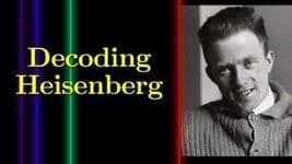
This is a step-by-step guide into Heisenberg’s famous «Umdeutung paper» in which he created quantum mechanics in 1925. I include the experimental reason for the need of matrices, a deep dive into the four key ideas of Heisenberg’s paper, and a detailed worked-out example showing how zero-point energy naturally appears in Heisenberg’s theory thanks to an early draft of what years later would become Heisenberg’s uncertainty principle.
*https://www.youtube.com/watch?v=oVzzIkkYGY8
**https://300.ya.ru/summary
таймкоды
00:00:02 Введение в квантовую механику Гейзенберга
- Вернер Гейзенберг разработал первую последовательную теорию квантовой механики в 1925 году.
- Его статья содержит четыре революционные идеи, которые переписали законы физики.
- Видео объясняет эти идеи, концепции и расчёты, чтобы показать, как Гейзенберг создал квантовую механику.
00:00:34 Цель видео
- Цель видео — сделать статью Гейзенберга более доступной, используя простые физические законы и математические выкладки.
- К концу видео будет объяснена энергия нулевых колебаний и принцип неопределённости.
- Видео разделено на три части: экспериментальный факт, основные идеи и пример из статьи Гейзенберга.
00:01:31 Экспериментальный факт и матрицы
- Теория Гейзенберга называется матричной механикой из-за использования математических массивов чисел.
- Эксперимент Вальтера Ритца в 1908 году показал закономерность в спектральных линиях водорода.
- Комбинационный принцип RITS объясняет, как частоты спектральных линий объединяются.
00:04:18 Исторический контекст
- Гейзенберг изменил старую квантовую теорию после уединения на острове в 1925 году.
- Эйнштейн ввёл вынужденное излучение и вероятности переходов в 1917 году.
- Латтенберг и Крамерс связали квантовые вероятности с классическими величинами в 1921 году.
00:06:12 Основные идеи Гейзенберга
- Гейзенберг предложил отказаться от ненаблюдаемых величин, таких как положение и период обращения электрона.
- Квантовая механика должна учитывать только взаимосвязи между наблюдаемыми величинами.
- Эта идея вызвала споры, особенно с Эйнштейном и Шрёдингером.
00:07:10 Представление о положении электрона
- Классическое движение электрона описывается рядом Фурье.
- Коэффициенты Фурье связаны с вероятностями переходов между состояниями.
- Гейзенберг заменил классические моды Фурье на амплитуды переходов.
00:09:01 Принцип соответствия
- Классическая частота орбитального движения заменяется на частоты переходов между состояниями атома.
- Положение квантового электрона записывается через амплитуды перехода.
- Положительные значения альфа соответствуют переходам между текущим состоянием и более низкими уровнями, отрицательные — более высоким уровням.
00:10:57 Движение и механика
- Гейзенберг начал с второго закона Ньютона, записав силу и ускорение как функции положения.
- Уравнение движения записывается в терминах квантовой координаты.
- Пример: для гармонического осциллятора F равно омега-ноль в квадрате, умноженное на x.
00:11:57 Умножение в квантовой механике
- Произведение двух координат в классическом случае даёт новый ряд Фурье.
- В квантовой интерпретации перемножение рядов Фурье не всегда даёт новый ряд из-за несоответствия индексов принципу комбинирования Ритца.
- Гейзенберг предположил, что квантовые объекты перемножаются иначе.
00:13:47 Принцип комбинирования Ритца и правило умножения Гейзенберга
- Гейзенберг использовал принцип комбинирования Ритца для преобразования суммы квантовых частот в одну новую частоту.
- Его правило умножения требует, чтобы второй индекс первой амплитуды был равен первому индексу второй амплитуды.
- Это правило позволяет легко складывать частоты в экспоненте.
00:14:42 Некоммутативность квантовых объектов
- Гейзенберг обнаружил, что квантовые объекты не являются коммутативными.
- Это открытие стало основой современной квантовой механики.
- Гейзенберг поделился своими опасениями с Максом Борном.
00:15:42 Матричное умножение и его открытие
- Ганс Бетте отметил, что соотношение Гейзенберга напоминает матричное умножение.
- Гейзенберг не знал о существовании матриц, но его результаты соответствовали матричной алгебре.
- Макс Баум объяснил Гейзенбергу, что его результаты — это умножение матриц.
00:17:23 Новое правило квантования
- Гейзенберг ввёл новое правило квантования, заменив классическое решение на амплитуды и частоты переходов.
- Он заменил импульс и координату их классическими разложениями в ряд Фурье.
- Новое правило позволило определить амплитуды и частоты переходов без использования классического решения.
00:20:14 Интерпретация правила квантования
- Гейзенберг интерпретировал правило квантования Бора — Зоммерфельда через амплитуды переходов и квантовые частоты.
- Он взял производную по квантовому числу n, что превратило классические производные в квантовые разности.
- Это позволило переформулировать квантовое правило на новом языке амплитуд и частот.
00:22:08 Ключевые концепции теории Гейзенберга
- Положение частицы описывается через амплитуды и частоты переходов.
- Амплитуды переходов определяют интенсивность спектра, а частоты — длину волны.
- Теория основана на законах Ньютона и позже была преобразована в гамильтонову теорию.
- Квантовые объекты подчиняются некоммутативному правилу умножения.
00:25:00 Применение метода Гейзенберга
- Пример негармонического осциллятора иллюстрирует применение метода Гейзенберга.
- Для понимания примера необходимо знать методы теории возмущений.
- Сравнение результатов с правилом Бора — Зоммерфельда показывает тонкие различия в подходах.
00:26:24 Решение задачи гармонического осциллятора
- Дифференциальное уравнение гармонического осциллятора имеет общее решение, где A и B — константы, а ω0 — основная частота осциллятора.
- В ряду Фурье ненулевыми являются только две гармоники, частоты которых кратны ω0.
- Квантовое решение подчиняется правилу квантования Бора — Зоммерфельда для гармоник Фурье.
00:27:18 Энергетические уровни квантового осциллятора
- Вычисление энергетических уровней с помощью разложения в ряд Фурье.
- Использование свойств комплексных чисел для получения общего выражения для гармоники Фурье.
- Подтверждение сохранения энергии: энергетические уровни не меняются со временем.
00:28:17 Соотношение Бора — Эйнштейна
- Энергетические уровни пропорциональны квантовому числу n.
- Разница между соседними уровнями энергии равна hbar * частота излучения ^n.
- Выполнение соотношения Бора — Эйнштейна.
00:29:15 Метод Гейзенберга
- Применение метода Гейзенберга для вычисления второй производной по времени.
- Определение частот и амплитуд переходов между состояниями.
- Правило отбора: разрешены только переходы между состояниями, отличающимися на одну квантовую единицу.
00:30:07 Рекурсивное соотношение для амплитуд
- Использование квантового условия для рекурсивного определения амплитуд.
- Определение основного состояния как состояния с наименьшей энергией.
- Нахождение амплитуд переходов для всех состояний.
00:32:00 Вычисление энергии осциллятора
- Применение правила умножения Гейзенберга для вычисления x’^2 и x^2.
- Разложение суммы по альфа и бета с учётом правил отбора.
- Вычисление частот переходов и получение выражения для кинетической энергии.
00:34:55 Сохранение энергии
- Подтверждение сохранения энергии гармонического осциллятора в квантовой механике.
- Окончательное выражение для энергии с учётом амплитуд.
- Выполнение соотношения Бора — Эйнштейна при условии равноотстоящих энергетических уровней.
00:35:47 Энергия основного состояния
- Энергия основного состояния составляет половину hbar * omega_0.
- Экспериментальное подтверждение энергии нулевых колебаний.
- Теория Гейзенберга объясняет остаточную энергию квантовых систем.
00:37:26 Принцип неопределённости
- Связь постоянного члена в формуле для энергии с новым квантовым условием.
- Преобразование нового правила в каноническое квантовое коммутационное соотношение.
- Принцип неопределённости Гейзенберга как следствие этого соотношения.
В этом видео
0:03
In the summer of 1925, Verer Heisenberg developed the first
0:08
consistent theory of quantum mechanics. The paper he wrote is cryptic even for
0:13
experts. But inside we find four groundbreaking ideas that rewrote the
0:19
rules of physics. In this video, I will walk you through these ideas, concepts,
0:24
and calculations to show you exactly how Heisenberg created quantum mechanics.
0:35
Quantum mechanics was created by Verer Heisenberg in 1925 with the publication
0:41
of this paper. The content is hard to follow. Some sections lack continuity
0:47
and some mathematical steps look like magic. The goal of this video is to change that and only with the help of
0:54
not very advanced physics and plenty of mathematical manipulation, I hope to make Heisenberg’s paper more accessible.
1:02
By the end of this video, we will discover how the famous 0 point energy appears in Heisenberg’s theory and an
1:10
early draft of what later became the uncertainty principle. In this
1:15
step-by-step guide, I will show you all the details so you can also enjoy the
1:20
beauty of this groundbreaking paper. This video is divided into three parts.
1:26
I will begin by showing you the experimental fact that led to matrices.
1:31
Then I will introduce the four core ideas and calculations in the paper. And
1:36
finally I will present one of the examples that Heisenberg provided at the
1:42
end of his paper including all the gory details that I hope can give you a glimpse on the work of theoretical
1:49
physics. As you probably know, Heisenberg’s theory of quantum mechanics
1:54
became known as matrix mechanics because of the use of these mathematical arrays
2:00
of numbers. I want to begin by answering one simple question. Why are matrices
2:06
needed in quantum mechanics? The answer is a simple experimental observation
2:11
made by the Swiss physicist Valter Ritz in the summer of 1908.
2:17
This table shows some of the lines of the hydrogen spectrum. Let’s take these
2:23
two and add their inverse. And now let’s look at the inverse of this line.
2:30
Let’s try with these lines. Now these three. There is clearly a
2:36
pattern here. One last time. I will now show you why this happens. This is a
2:44
formula that Reitberg found in 1888 for the wavelength of hydrogen spectral
2:50
lines in terms of two integer numbers J and K. R is just a constant. Multiplying
2:56
all this by the speed of light, we get frequencies instead. Notice what happens
3:02
when we add two frequencies in which the second index of one is identical to the
3:09
first index of the other. Using the formula above, we find that the middle
3:14
indices cancel out and we get a new frequency with the first index of one
3:20
and the second index of the other. This relation is a general result for spectral lines. And this is exactly what
3:27
I show you in the examples. If I include the indices, you can see that in all
3:33
cases, the general formula works. This relation is an example of the so-called
3:39
Ritz combination principle and it tells us how the frequencies of a spectral
3:44
lines are combined to form new frequencies. This observation is the key
3:50
to unlocking the ideas in Heisenber’s paper. And as I will show you shortly,
3:55
this experimental fact is the reason for the need of matrices.
4:01
Since 1900, quantum physics was a collection of arbitrary and unjustified
4:07
rules that became known as old quantum theory. Heisenberg changed all that
4:13
after an isolation retreat in a remote island in June 1925.
4:19
After his return, he wrote a cryptic paper titled on the quantum theoretical
4:25
reinterpretation of kinematical and mechanical relationships in which he laid out four rules for calculating the
4:32
outcome of experiments. Everything began with Einstein’s quantum theory of radiation from 1917. After
4:40
completing his monumental work on general relativity, Einstein returned to the study of radiation, introducing two
4:48
key innovations, a new process called stimulated emission and transition
4:53
probabilities for describing the absorption and emission of light. Unfortunately, there was no way to
5:00
determine these probabilities. The breakthrough came in early 1921 when
5:05
Rudolfph Latenburgg found a way to connect Einstein’s quantum probabilities
5:10
with classical quantities that could be measured in dispersion experiments. Inspired by Latenburg, this idea was
5:18
extended by Henrik Kramers who found a quantum theory of dispersion. Kramers
5:24
and Max Bourne also discovered a mathematical relation between classical
5:29
and quantum relations that was crucial for Heisenberg. Let’s now dive into
5:34
Heisenberg’s famous paper. The key word is reinterpretation.
5:39
Historians of science refer to this work as the unon paper. What everyone was
5:45
searching for during the 1920s was a way to derive quantum equations to replace
5:51
the equations of classical mechanics. Heisenberg built on the ideas of Einstein, Latenburg, Kmers, Bore and
5:59
Bourne to find the quantum equivalent of physical quantities from a classical
6:05
theory. He starts by setting one of the core ideas in which his quantum
6:11
mechanics is built. It is advisable to completely discard unobserved quantities
6:17
such as the electrons position and period. Instead, it seems more
6:22
reasonable to try to establish a theory of quantum mechanics in which only relationships among observable
6:30
quantities occur. This is one of the most radical ideas in the history of physics, one that leads to debates even
6:37
today. Heisenberg proposes here that quantum mechanics is only a theory about
6:43
experimental observables. In his paper, these are the transition amplitudes and
6:49
frequencies. Although this idea is usually attributed to Heisenberg, one of
6:54
its main proponents was Wol and Powley. His letters show that by the summer of
7:00
1925, he had convinced most of the key figures of quantum theory about this
7:05
idea. This is something that Einstein and Shinger strongly opposed. For them,
7:11
physics is about describing nature as a whole, including all its underlying
7:16
mechanisms, even those that we cannot measure. We could say that with this
7:21
sentence, Heisenberg began the infamous shut up and calculate approach. Let me
7:27
know in the comments if you have an opinion about this idea. After this, Heisenberg begins his rumblings. I stop
7:35
following the paper here and present the ideas in a more coherent order pointing out to the corresponding results in the
7:41
paper. The first concept is position. The classical view of the electron
7:47
orbiting the nucleus was enough for atoms with a single electron but failed
7:52
with all the others. After his work with Bourne, Heisenberg knew that a classical
7:58
periodic motion of an electron in a stationary state n can be described as
8:04
an infinite sum of oscillations. This is called a furier series. A more general
8:11
way to write this is by using a complex exponential instead where the sum is
8:16
over all positive and negative values of the index alpha. I will later drop the
8:22
estimation range to simplify notation. The factors a alpha are called fura
8:28
modes and kramers showed in his doctoral thesis that these factors are directly
8:34
related to the transition probabilities between states introduced by Einstein in
8:39
his paper on quantum radiation. The position is a real quantity. Forcing all
8:45
this sum to be equal to its own complex conjugate implies a relation between the
8:51
negative and positive fura modes. This relation will be very useful later. Here
8:57
heisenberg introduces his first seminal idea. According to the correspondence
9:03
principle, the classical frequency of the orbital motion of the electron and
9:08
its harmonics get replaced by the transition frequencies between atomic
9:13
states. Alpha omega becomes omega and k where n is the current state of the
9:19
electron and k is any other state that the electron can transition via a
9:25
quantum jump. Just for clarity in this video, I will use the subindex k as
9:31
short notation for n minus alpha. Now we can write the position of the quantum
9:37
electron in this way where the classical furier modes are replaced by transition
9:43
amplitudes with two indices to match the transition frequencies that obey the
9:48
ritz combination principle. Just like in the classical case, forcing the position
9:53
to be a real quantity implies this relationship. Reversing the indices of
9:59
the amplitudes is equivalent to checking its complex conjugate. This relation
10:05
corresponds to Heisenber’s position reinterpretation and the word kinematics
10:10
in the title of his paper. Note that the positive values of alpha represent
10:16
quantum transitions between the current state n and lower levels whereas the
10:22
negative values denote higher levels. With this expression, Heisenberg built a
10:27
tower of so-called virtual oscillators. The next concept is motion. I bet many
10:34
of you were not expecting to find Newton’s second law in the foundational paper on quantum mechanics, but this is
10:41
Heisenberg’s starting point. Writing the force and acceleration as functions of
10:47
position, dividing by the mass of the particle and collecting terms on the
10:52
left hand side. Heisenberg renamed this ratio just f. His idea is that depending
10:59
on the physical system of interest, all you have to do is to identify the potential energy, calculate f and
11:07
properly write this equation of motion in terms of the quantum position as defined in the previous section. This
11:14
concept is the mechanics in the title of his paper. as examples for the harmonic
11:21
oscillator f is just omega^ squar * x
11:26
whereas the so-called unharmonic oscillator has an extra term with x
11:31
squared in general for any function we can expand the function as a power
11:37
series of x and here realized that we need a proper definition of how to
11:44
calculate powers of x which takes us to the third concept Multiplication.
11:50
This concept is probably the most important and revolutionary in the paper. Back to the classical
11:56
definitions. Let’s see what the product of two positions X and Y is in terms of
12:02
FIA modes. For this, we simply multiply two FA series where A are the modes of X
12:09
and B are the modes of Y. Note that the exponential now combines harmonics of X
12:16
and Y. However, we can introduce a new index toao which allows writing the
12:21
product as a new fier series. Defining the new fier modes in terms of a and b,
12:28
we explicitly find that the product of two positions x and y gives a series
12:34
that has the same structure as x. This is one of the great properties of a
12:39
series. We can calculate the product between y and x instead. Following the
12:45
same steps as before, we find that the order of the product makes no difference. We call quantities that
12:52
satisfy this relation commutative objects. A common example is real
12:57
numbers. The order of the factors does not affect the product. Now we repeat
13:03
this but using the quantum reinterpretation of position and frequency introduced before. Taking
13:10
their product, we must be careful with the indices. And just like in the classical case, the two corresponding
13:16
frequencies appear added in the exponential. But now we have a problem. Note that the two frequencies cannot be
13:24
combined into a new frequency like in the classical case because the indices do not match the RIT’s combination
13:31
principle. This would mark the end of Heisenber’s efforts because the product
13:36
of two series does not produce a new series. But here comes the bold move.
13:42
Heisenberg proposed that this is not how quantum objects are multiplied. He wants
13:48
the two frequencies in the exponential to have the indices in such order that the rich combination principle can be
13:55
used to convert this sum of quantum frequencies into a single new frequency.
14:01
Remember that the ritz combination principle is an experimental fact. Heisenber simply took this feature of
14:07
nature and used it to invent a new way to manipulate transition frequencies.
14:13
His multiplication rule is that the second index of the first amplitude must
14:20
be equal to the first index of the second amplitude. In this way, the two
14:25
frequencies in the exponential can be easily added using the Ritz combination principle. Now we proceed just as
14:33
before. We rename the product of amplitudes and find that the product of these two quantum objects is a series
14:41
like the original. We can repeat the same steps to calculate y * x instead.
14:47
But now we find that the indices are arranged in a way that the two products are except in very special cases not
14:55
equal. Here Heisenberg found that a consequence of his quantum reinterpretation is that quantum objects
15:03
are not commutative. This is the bold conceptual innovation that makes this
15:08
paper the foundation of modern quantum mechanics. This weird multiplication
15:14
rule made Heisenberg very uncomfortable. In the paper he wrote this
15:19
multiplication rule is an almost necessary consequence of the frequency combination rules. He accepted what his
15:27
theory was telling him but could not make sense of the meaning of these non-commutative objects. After his
15:34
return from Helgoland, he expressed his concern to Max Bourne. What are these
15:39
objects that obey these rules? Let me bring back the way the transition amplitudes are combined. Heisenberg was
15:47
baffled by this relation. But today, even a freshman student would recognize
15:52
it as matrix multiplication. Believe it or not, Heisenberg didn’t know about
15:57
matrices. This is how Hans Bete, one of the great students of Somerfield and
16:03
Heisenberg, described it. So he said we should only talk about
16:09
experimentally observable quantities both the frequencies and these
16:14
amplitudes but should forget about the motion of electrons in orbits.
16:24
Then he discussed just how these quantities Q
16:31
and PKN should occur in the theory. how would you form kinetic and potential
16:37
energy from them? And he found that these uh quantities obeyed very strange
16:44
multiplication rules which he had never seen before. But he wrote down these
16:50
multiplication rules. Uh P and Q just did not uh behave like ordinary
16:57
algebraic quantities. when he came home to Guttingan
17:02
uh Max Bon told him but Heisenberg what you have there is simply the multiplication of matrices.
17:09
Now you all learn about matrices probably in your freshman year or at
17:15
most in your sophomore year but Heisenberg had never heard about matrices.
17:24
Thanks to Bourne, Heisenberg discovered that quantum objects follow the rules of
17:29
matrix algebra. But this only happened after he wrote his paper. Before we
17:35
judge Heisenberg for not knowing about matrices, the same was true for most physicists of the time. Matrix algebra
17:43
was so unknown that the paper that Bourne and Jordan wrote following on Heisenber’s work began with a full
17:50
section explaining the basics of matrices. The fourth and final concept introduced
17:57
by Heisenberg was a new quantization rule. I remind you that old quantum
18:02
theory was mostly based on the rule developed by Bore and Somerfeld. This
18:08
was very successful for describing an isolated hydrogen atom, but it failed in
18:14
light of new experiments. This rule worked as follows. First, write the
18:20
classical equation of motion. then solve the equation to find the classical solution and finally force the classical
18:28
solution to satisfy the bore summerfeld rule. In Heisenber’s approach, the
18:33
classical solution is irrelevant because the goal is to determine the transition amplitudes and frequencies. For this
18:40
reason, a new quantization rule was needed. Heisenberg took the rule from old quantum theory and replaced momentum
18:48
and position by their classical FA expansions. Using the chain rule, the
18:53
integral over position can be turned into an integral over one orbital
18:59
period. We need to determine x dot squared. Since we know x, we can
19:04
directly take the time derivative and then take the product with itself. These
19:10
are classical free expansions. So this is the conventional product. Now we can
19:16
use a trick. Since the sum over beta includes all positive and negative
19:21
values, we can replace beta by minus beta in this expression and the sum does
19:27
not change. In this line, I have simply replaced every beta by minus beta. Now
19:33
we can integrate over time. The orbital period is related to the frequency. So
19:39
we can make this change of variables. This angular integral is not trivial but
19:44
it happens to vanish except when beta is equal to alpha. In case you are familiar
19:50
with the name this is an integral representation of the chronicer delta.
19:56
This means that when summing over beta all terms are zero except when beta
20:02
equals alpha and this expression reduces to a single sum. There is nothing new
20:09
here. This relation is just the bore summerfell rule for fier modes. Now
20:14
Heisenberg tried to reinterpret this relation. The obvious thing to do is
20:19
replacing the fier modes and harmonics frequencies by transition amplitudes and
20:25
quantum frequencies respectively. However, there is a problem. What to do with this extra index alpha?
20:32
Heisenberg’s reinterpretation of frequency only eliminates one of the alpha indices. meaning that a direct
20:40
reinterpretation of the bore summerfeld rule is not possible. Here is
20:45
Heisenberg’s workaround. He took the derivative with respect to the quantum
20:50
number n on both sides. This expression looks even more complicated. But here he
20:56
invoked what we could call the reinterpretation discovered independently by Bourne and Kmers. This
21:03
relation turns classical derivatives into quantum differences.
21:08
This is one of the great outcomes obtained in the spirit of the failed BKS theory that I presented in a previous
21:15
video. Using this relation, Heisenberg was able to transform the quantum rule
21:21
of the old quantum theory into his new language of transition amplitudes and
21:26
frequencies. Heisenber understood that this rule provides a recursive relation
21:32
between amplitudes. Once you know the amplitude for one quantum transition,
21:37
this relation allows finding the others. This formula and the equation of motion
21:43
with the corresponding multiplication rule constitute the equations of Heisenberg’s quantum theory. And these
21:50
are the revolutionary ideas in the paper. Here is a summary of the key concepts in Heisenberg’s paper. Position
21:58
is written in terms of transition amplitudes and frequencies. These two quantities are the central unknowns of
22:04
the theory because they are observable in experiments. The transition amplitudes define the intensity of the
22:11
spectral lines and the frequencies determine their wavelength. Motion is characterized by the quantum
22:18
position object satisfying the classical equations. Note that Heisenberg’s theory
22:24
is Newtonian. This was later improved and turned into a more general
22:29
Hamiltonian theory by Heisenberg in collaboration with Bourne and Jordan.
22:34
Maybe I should make a video about that too. Quantum objects obey an unusual
22:39
multiplication rule. Non-commutativity of quantum quantities is one of the
22:44
central discoveries in the paper. Thanks to Bourne, Heisenberg and the rest of the physics community learned that
22:51
transition amplitudes are described by matrix algebra and Heisenberg’s theory
22:57
became known as the matrix formulation of quantum mechanics. The quantum nature of transition
23:03
amplitudes and frequencies is specified by Heisenberg’s reinterpretation of the
23:09
old Bore Somerfell quantum rule. Here is where plank’s constant enters the
23:14
equations. And that’s it. This is the recipe for a self-consistent and
23:20
systematic quantum mechanics. Heisenberg described it like this. Equations 11 and
23:26
16 contain a complete determination not only of frequencies and energy values
23:32
but also of quantum transition probabilities. The paper also includes two crucial
23:38
questions probably influenced by the recent reputation of BKS theory.
23:44
Heisenberg wondered about energy conservation and also whether the energy levels predicted by his theory would
23:51
satisfy the wellestablished bore Einstein relation. But the only way to
23:56
answer these questions was by testing the theory with examples. This is what I
24:02
will do in the next part. Heisenberg’s method was a first draft
24:07
for quantum mechanics. All the main ingredients are there, but he knew that a mathematical refinement was needed. He
24:15
ended his paper with an invitation to such mathematical polishing of his ideas. Whether the method proposed here
24:22
can be regarded as satisfactory can be decided only by more intensive mathematical investigation. The method
24:30
has been very superficially employed here. In the last section of this video, I
24:36
want to show you an explicit example of how to use Heisenber’s idea to a
24:41
particular system. Although I will present a simplified case, I will include all the gory details because I
24:49
find this a very instructive exercise. I honestly think that I understood the main ideas in Heisenberg’s paper only
24:56
after going through these calculations and I hope that they can help you too. This would let you appreciate the amount
25:02
of work behind every result in the paper and hopefully give you a glimpse of the work of a theoretical physicist.
25:09
Heisenber begins section three of his paper with as a simple example the
25:16
anharmonic oscillator will now be treated. The interest in the unharmonic
25:21
oscillator is that just like the hydrogen atom transitions between all levels are possible. However, this
25:28
example requires familiarity with the methods of perturbation theory. Since I
25:33
want this exercise to be valuable even if this is your first encounter with quantum mechanics, I will only cover the
25:41
particular case of lambda equals 0. This is the simple harmonic oscillator. There
25:46
is a running joke that the simple harmonic oscillator is the only system that physicists know how to solve.
25:53
Sydney Collan described it better. The career of a young theoretical physicist
25:58
consists of treating the harmonic oscillator in everinccreasing levels of abstraction. And if you have studied
26:04
quantum mechanics and quantum field theory, you know that this is true. I will first solve this using the bore
26:12
Somerfell rule of the old quantum theory and then using Heisenber’s quantum mechanics so we can compare. If you
26:20
watch my last video, you will like the subtle differences. As you probably know, the differential
26:27
equation of the harmonic oscillator is exactly satisfied by this general
26:32
solution where a and b are constants and omega kn is the fundamental frequency of
26:38
the oscillator. Comparing this solution with the general fier series, we
26:43
immediately find that there are only two nonzero fier modes and the harmonics are
26:49
given by multiples of omega kn. This means that the infinite sum only has two
26:55
terms. Following the recipe of old quantum theory, now that we have found a
27:00
classical solution, we make it quantum by forcing it to obey the bore summerfield rule for fier modes found
27:08
before where n is an integer. Let’s not forget that this sum has only two terms.
27:15
One for alpha= 1 and alpha= minus1. by properties of complex numbers. This
27:21
reduces to a single term from which we directly find the general expression of
27:27
the only nonzero fier mode. Let’s now calculate the energy levels of this old
27:32
quantum oscillator. Note that we need to determine x dot squared and x². And for
27:40
this we use our simple fa expansion. X dot is given by this. And it’s a square
27:46
leads to three terms. Then we do the same for x^2. The calculation is very
27:52
similar. Plug in these two quantities in the expression for energy, we have six
27:58
terms, but two pairs cancel each other out while the other two are identical.
28:04
Note that all time dependence disappears, meaning that the energy levels are constant in time. Energy is
28:12
conserved. We have found the energy levels in terms of the fier modes. We
28:17
can now replace our previous result to find that the energy levels are proportional to the quantum number n.
28:25
For this reason, the energy gap between two adjacent levels is exactly h bar
28:30
omega kn and the bore einstein relation is satisfied. Here is the summary of the
28:37
results. Now we repeat this but following method.
28:42
Just like before, we begin with the quantum position, but instead of using the classical solution, we calculate the
28:49
second time derivative to replace it into the equation of motion. Factorizing
28:54
common terms, we find this relation. From now on, we will need the complete form of the indices. So, I am replacing
29:02
K by N minus alpha. Under the assumption that every state has its own energy for
29:10
each value of alpha in the sum, the exponent will be different. This means
29:16
that each element of the sum must individually vanish. For alpha equals 0,
29:22
we get this. Since the transition frequency of a state with itself is
29:27
zero, we find that the same is true for the amplitude. For alpha equals 1, we
29:34
get this. Inspired by the classical result, we set the amplitude between one level and the next to be non zero, which
29:41
gives us a constant value for the transition frequency. Contrary to the
29:46
hydrogen atom, here the frequencies are independent of the quantum number n,
29:52
which means that the energy levels are equally spaced. We can now repeat for
29:57
alpha= minus1 to get this. Just like the classical case, the only nonzero
30:04
transition amplitudes are between adjacent states. Using that the energy levels are equally spaced implies that
30:12
for all other values of alpha, the amplitude is zero. Summarizing from the
30:18
equation of motion, we found the frequencies and the nonvanishing amplitudes. This condition that the only
30:26
allowed transitions are between states that defer by one quantum unit is
30:31
usually known as selection rules. We still need to find the value of these two amplitudes. For this, we use the
30:37
older equation in Heisenberg’s method, the quantum condition. As mentioned
30:42
before, this equation provides a recursive way to determine the amplitudes. Since alpha can only take
30:49
two values, we can expand the sum leading to four terms. Using the previous result for the transition
30:56
amplitudes and being extra careful with the order of the indices to get all the signs right, we find that the four terms
31:04
reduce to two terms. Finally, we can write the recursive relation for the
31:09
amplitudes. The next step is defining a so-called ground state. This is defined
31:16
as the lowest possible state of the system. Setting this to be represented
31:21
by n equals 0, we get the following. In this step, heisenber reasoned that
31:28
transitions below the level n= 0 do not exist by definition of ground state.
31:35
Therefore, this term must be zero. And with this, we find our first transition
31:41
amplitude. Next we take n= 1 which is given in terms of the transition that we
31:47
just found. We can repeat for n= 2 and quickly find the pattern for any state
31:54
n. This is the transition amplitude which I will add to the summary on the
31:59
top right. Note that the absolute value allows reversing the state indices
32:05
without affecting the result. Also notice that we can replace n by n minus
32:11
one to obtain this pair of relations that will be useful in a minute. The
32:17
final calculation is the energy of the oscillator. Just like before we need to determine x dot squar and x^2. But this
32:26
time we must use Heisenber’s multiplication rule. For x dot we simply
32:32
take the derivative with respect to time. Here notice that all these terms
32:38
correspond to the amplitude that we have to use in the multiplication rule. The
32:43
product of x dot with itself gives us this long expression. Now we use that
32:50
only transitions between adjacent states are allowed to expand the sum over
32:55
alpha. So we get two terms for the sum over beta. We have to be extra careful.
33:01
Let’s look at this term from the selection rules. The indices in the amplitude can only defer by one.
33:09
Therefore, beta can only take the values zero or two leading to these two terms.
33:16
Using the same method with the second term, we find that beta can only take
33:21
the values 0 and minus2 producing the next two terms. Now we have to evaluate
33:28
the frequencies. Since the two amplitudes have the same indices in
33:33
reverse order, their product is just the squared magnitude. Using our previous
33:39
results, the first frequency is positive and equal to omega KN. Whereas the
33:44
second frequency has the same indices in reverse order. So it has an extra minus.
33:50
Finally, we use that the transition frequency of a state with itself is zero. Just to make sure that the method
33:57
is clear, let me do the second term. Here the product of amplitudes remains
34:02
as it is. The first frequency is again omega kn whereas the second frequency is
34:08
also omega kn. If this is unclear, just replace n by n minus one in the formula
34:14
above. The exponent is no longer zero. Since we know that the energy levels are
34:20
equally spaced, the frequency between levels two units apart is simply two
34:25
times omega KN. Using the same procedure with the other two terms, we get this.
34:32
Taking out the common factor omega squared, we have found the expression
34:38
needed for the kinetic energy. The same steps are needed for x^2. We expand the
34:44
sum over alpha, then sum over beta and evaluate the frequencies. This is much
34:50
easier than the previous one. And now we’re ready to calculate the energy of the oscillator. Like the semi-class
34:57
case, all the time dependent terms cancel each other out, making the energy
35:02
levels constant. This answers Heisenberg’s question about energy conservation. Yes, the energy of the
35:10
harmonic oscillator in quantum mechanics is conserved. Now I bring back the
35:15
amplitudes that we found before because we can determine the final expression for the energy. Plugging the two
35:22
relevant amplitudes, we get this. Factorizing common terms, we finally
35:28
find the energy. Here is the summary of all the results that we found. We can
35:34
answer Heisenberg’s second question. Yes, given that the energy levels are equally spaced, the bore Einstein
35:41
relation is satisfied. This is the final answer from Heisenberg’s point of view.
35:47
It is not the position of the oscillator or its speed but the observable
35:53
quantities transition amplitudes and frequencies. Additionally, we find that the energy of
36:00
the ground state is not zero, but 1/2 h bar omega kn exactly as many experiments
36:07
indicated. In case you’re unfamiliar with this, make sure to check my video about the 0 point energy. In that video,
36:15
I mentioned that there was no room for this factor 1/2 h bar omega in quantum
36:20
theory before Heisenberg. Bringing back the results of the semic-class theory of
36:25
the harmonic oscillator, we see that Heisenber’s theory agrees with all the results of the bore summer theory except
36:34
for the 0 point energy. In the old theory, the energy of the ground state n
36:39
equals 0 is exactly zero. in contradiction with many experiments at
36:44
low temperatures that show that quantum systems exhibit a remnant energy of 1/2
36:50
h bar omega. The hope was that a systematic theory of quantum mechanics
36:56
could explain the origin of this residual energy and Heisenberg’s quantum mechanics did exactly that. If you track
37:04
the origin of the constant term in the energy, you will find it to arise from
37:09
the new quantum condition. Bourne and Jordan transformed this new rule created
37:14
by Heisenberg into one of the fundamental building blocks of quantum mechanics found today in textbooks. The
37:21
so-called canonical quantum commutation relation from which the famous Heisenberg’s uncertainty principle can
37:28
be derived. But this happens two years later. For now, I wanted to show you that Heisenberg’s paper already contains
37:36
many of the blueprints for modern quantum mechanics. And although he didn’t know it, this formula is the
37:43
first draft of his famous uncertainty principle. If you made it this far, congratulations
37:51
and thank you for joining me. This is a remarkable paper and I hope that with
37:56
this deep dive any student even at the undergraduate level can understand its
38:01
significance and reproduce the original calculations. Most textbooks present
38:07
these results as coming out of a magic hat but in reality they can be derived
38:12
using some math a good understanding of the historical context and more
38:17
importantly building out of experimental evidence.